Accessing the Anki database from R

Posted on February 3, 2018 | Reading time 8 minutes

key points

We will get the Anki database data into R

Introduction and prerequisites

Anki uses a SQLite database, in order to store all your notes, settings, reviews, etc. I’ve always wanted to mess around with the review data, and create some charts with it. I assume that you know some basic R or SQL. Even if you don’t, I think you’ll be fine if you have some understanding of programming languages, as the code presented here is far from complicated.

In order to have a save working environment, I strongly recommend working on a copy of your database. You can find it (on Windows) in %appdata%/anki2/YOUR_PROFILE. Copy the file collection.anki2 to a new folder, and create a .R script in the same location. I tend to use RStudio as my environment when coding, since it has some nifty features (e.g. run the selected line with Ctrl + R and inline documentation view). In RStudio, you can also set the working directory to the location of your code file via Session → Set Working Directory → To Source File Location

I will use the following packages in sections below: RSQLite, DBI (both to access the database), jsonlite (to parse some data) and ggplot2 (to create some graphs). If you don’t have experience with ggplot2, you might want check out this short introduction.

You can install the required packages and dependencies by running the following command:

1
install.packages(c("RSQLite", "DBI", "jsonlite", "ggplot2"))

Now obviously, we want to load these packages:

1
2
3
4
require(RSQLite)
require(DBI)
require(ggplot2)
require(jsonlite)

Getting data into Anki and resolving the deck names

The database contains the tables cards, col, graves, notes, revlog, sqlite_stat1. We will only import cards, col, notes, revlog, since they contain the most interesting data. In the following code, I won’t even access all tables. However, you will have every table ready to explore them further.

A detailed outline of the database can be found via the Anki Android wiki, which is linked at the end of this post.

I tend to import data as-is, and do the manipulation in R. So I will use import * from TABLE statements. To achieve certain things, you might also want to JOIN certain stuff directly.

 1
 2
 3
 4
 5
 6
 7
 8
 9
10
11
12
13
14
15
16
17
18
19
connection <- dbConnect(SQLite(), dbname="collection.anki2")

result <- dbSendQuery(connection, "SELECT * from cards")
cardData <- dbFetch(result)
dbClearResult(result)

result <- dbSendQuery(connection, "SELECT * from col")
collectionData <- dbFetch(result)
dbClearResult(result)

result <- dbSendQuery(connection, "SELECT * from notes")
notesData <- dbFetch(result)
dbClearResult(result)

result <- dbSendQuery(connection, "SELECT * from revlog")
revisionData <- dbFetch(result)
dbClearResult(result)

dbDisconnect(connection)

You will end up with four data frames, containing all the data from the database. We will start by exploring the collection dataframe. Running str(collectionData) shows us the structure:

 1
 2
 3
 4
 5
 6
 7
 8
 9
10
11
12
13
14
'data.frame':	1 obs. of  13 variables:
 $ id    : int 1
 $ crt   : int 1477461600
 $ mod   :integer64 1517651707090 
 $ scm   :integer64 1516989662176 
 $ ver   : int 11
 $ dty   : int 0
 $ usn   : int 724
 $ ls    :integer64 1517651707090 
 $ conf  : chr "{\"nextPos\": 5131, \"estTimes\": false, \"activeDecks\": [1511615148492, 1511615155451, 1511615353208, 1511615"| __truncated__
 $ models: chr "{\"1477567528678\": {\"vers\": [], \"name\": \"Basic\", \"tags\": [\"KLinische_Pharma_COPD\", \"Klinische_Pharm"| __truncated__
 $ decks : chr "{\"1485866371701\": {\"desc\": \"\", \"name\": \"Klinik::Psychosomatik\", \"extendRev\": 50, \"usn\": 723, \"co"| __truncated__
 $ dconf : chr "{\"1\": {\"name\": \"Default\", \"replayq\": true, \"lapse\": {\"leechFails\": 8, \"minInt\": 1, \"delays\": [1"| __truncated__
 $ tags  : chr "{\"Gyn_Gutartige_EndometriumCA\": 0, \"Derma_Allgemein\": 0, \"Sono\": 0, \"Uro\": 0, \"Innere_EKG\": 0, \"Uro_"| __truncated__

The most interesting entry here is the decks column. It contains a JSON representation of all our decks. Let’s extract this, and parse the JSON:

1
collectionNames <- fromJSON(txt=collectionData$decks[1]) # use the first row in the 'decks' column

The collectionNames contains a named list, allowing us to access deck data based on id. For instance, we can use collectionNames[["1"]] to access information about the default deck. Let’s create a function, that performs a lookup of the deck name based on the deck id.

1
getDeckName <- function(x) collectionNames[[x]]$name

We can now pass the deck id (as string), and will get the deck name as a result. Let’s put this to use.

The cardData data frame contains a column did, which contains the deck id of every card. Let’s add a column with the name of the deck of the card as well:

1
cardData$deck <- factor(mapply(getDeckName, as.character(cardData$did))) #perform lookup of deck names

What happens above: we apply the getDeckName function to each deck id. Before passing the ids, we convert them to a character (which is similar to a string data type from other languages). The results are turned into a factor, which categorizes your data. Every deck is a category, and every card can only be in one category. This step helps further on with graphing. Graphing library often times can’t make sense of text. But we now state, that the deck names are actually categories, plotting libraries can correctly interpret this data.

It might also be interesting to add card related data to the revisions. The revisions contain a log, for each card you have reviewed. The cid column is the card, that has been reviewed. Let’s also add the deck name to the revisions. We have to handle the case, where a card might have been removed. In this case, we will set “Removed card” as the deck name

 1
 2
 3
 4
 5
 6
 7
 8
 9
10
11
12
getDeckNameFromCid <- function(x)
  {
    lookup <- as.character(cardData$deck[cardData$id == x])
    
    if(identical(lookup, character(0))) #due to deleted cards, some lookups might fail
    {
      lookup <- "Removed card"
    }
    
    return(lookup)
  }
revisionData$deck <- factor(mapply(getDeckNameFromCid, revisionData$cid))

Depending on the amount of reviews, the lookup might take a while.

Let’s plot some stuff

Ok, so let’s get some plots going. First, let’s check out, let’s see how our review times fare. The time column in the revisionData tells us, how long we spent on every single answer. It actually contains the milliseconds, so we can just divide it by 1000 to get the seconds. I opted for a logarithmic y axis, since I had a huge number of reviews in the lower review times.

1
ggplot(revisionData, aes(time / 1000)) + geom_histogram(binwidth = 10) + xlab("Time spent reviewing a single card\n(seconds)") + scale_y_log10()

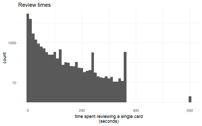
You can see, the time spent on each review seems to exponentially decrease, i.e. I do a lot of reviews in a few seconds, and only a hand full really take long. Also note, that the time cuts off at the level specified in the deck options, which I have set to 360. I also had it set to 600 some time ago.

Now, I’m interest in breaking this data up into my different decks. I will also limit the x-axis to the range containing the most data (0 to 400).

1
ggplot(revisionData, aes(time / 1000)) + geom_histogram(binwidth = 10) + xlim(0, 400) + xlab("time spent reviewing a single card\n(seconds)") + scale_y_log10() + ggtitle("Review times") + facet_wrap(~ deck)

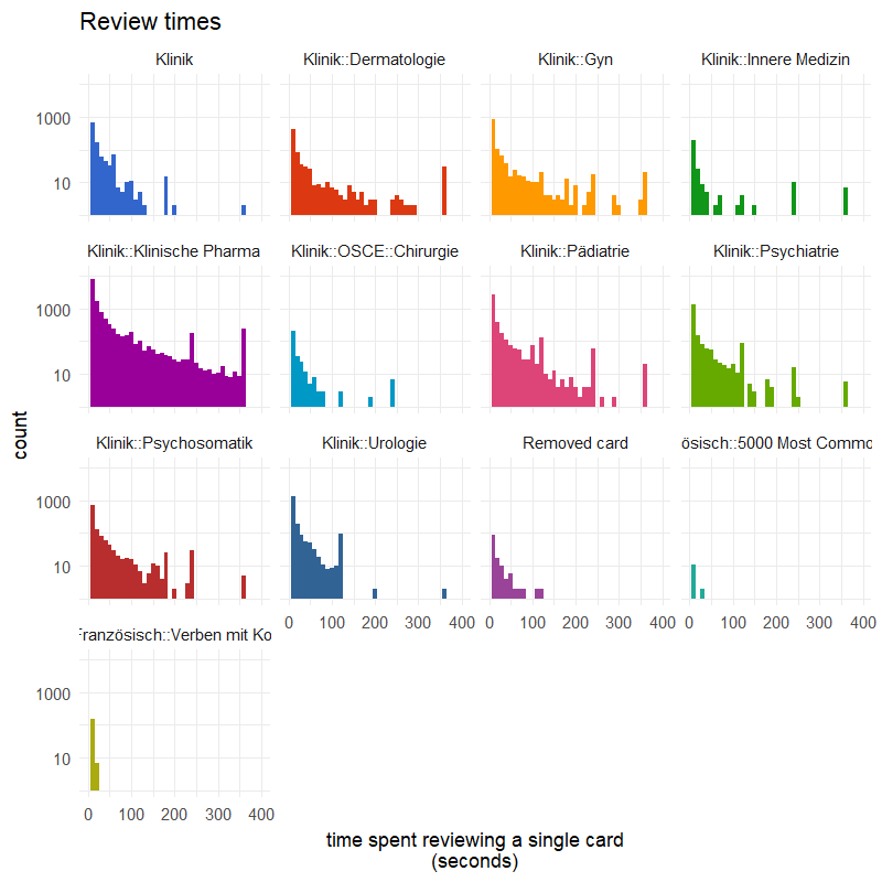
The purple deck was used for my last exam, where I used Anki extensively. This is easily recognizable by looking at the distribution. The review times stretch out further. For my surgical OSCE (light blue), I only had a small amount of very simple cards, therefore cards are much more clustered to the left. The bottom right and left (greenish and brownish) are language related, and I study them only for fun. Cards are only vocabularies, and are recalled very fast.

Finally, let’s see how our decks are composed. I want to check out, how my intervals are distributed across my different decks:

1
ggplot(cardData, aes(ivl)) + geom_histogram(binwidth = 10) + facet_wrap(~ deck, scales = "free_y")

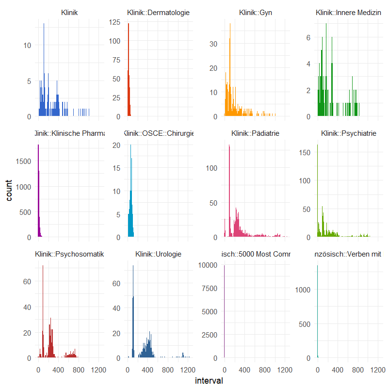
Note the free scales on the y-axis. The blue deck (top left), and the four top right ones (orange, pink, green and green) are older decks. You can see, how they have rather long intervals. Again the purple deck from my last exam. The cards are still very young here, indicated by the low intervals. My language decks have a huge number of cards, and I recently started with them. This is why they only have very low intervals.

How many cards are mature?

There was an idea on Reddit, to have a heatmap of every single card, with the interval color coded. This way, you could have a graphical representation of your progress. This is also possible with R.

1
2
3
4
5
6
plotWidth <- floor(sqrt(nrow(cardData))) # our final dimension should be a square
cardData$index <- (0 : (nrow(cardData) - 1)) # to calculate the position of each card, we need a running count
cardData$X <- cardData$index %% plotWidth # x position
cardData$Y <- cardData$index %/% plotWidth # y position
cardData$mature <- cardData$ivl > 21 # you can also use this, to show mature cards
ggplot(cardData, aes(X, Y)) + geom_tile(aes(fill = ivl)) + scale_fill_gradient2(mid = "#dd6a27", high = "#12e824")

As you can see, I have still a long way to go, until all my cards are mature. This is due to the large premade language decks I’ve imported. Below, I’ve filtered the premade decks out, and you can see a large red chunk disappears

Summary

We have imported the Anki data into R. By using only a fraction of the available data, we were able to get some insights into the data. The full code to create these graphics is available on GitHub here.

If you create a cool graphic, let me know via Twitter.

Here is another thing I’ve come up with. I’ve animated how the intervals of my cards have changed over the time. In the beginning, the maximum interval was quite limited. Once I’ve lifted that, you can see the intervals exploding. This was also done purely in R (and ffmpeg to get the video).