Bit depths, image data and histograms
Posted on October 9, 2016 | Reading time 9 minutes- You will understand how image information is represented as digital information
- You will understand the differences between different bit depths
- We will take a short introduction to histograms
Bits and numbers
Your computer actually knows only two states: 0 and 1. A bit is a storage that can either have the state 1 or 0 and is the smallest digital unit. Everything that is processed has to be represented by a chain of zeros and ones — a combination of bits. The actual information is received, when interpreting these bits in a certain way.
Let me give you an example: 562. Without context, you can’t really do anything with 562. But if I would tell you, that this is an office number, the 562 suddenly has a meaning. It could also be the extension of my phone number. And suddenly 562 has a different meaning.
Similarly, the values 0100100001101001 could either be interpreted as Hi, if you treat it as text. But it could also mean the decimal number 18537. We can see two things: a) we need to transform every information into combinations of 1 and 0, in order to process this information digitally; b) we need to define certain rules how to interpret data.
What is an image
A digital image is in its simplest form an arrangement of pixels. Every pixel stores information about the color at that place. Let’s think of the image as table. The following table could for instance create the image below (the displayed image is scaled up). Try to figure out what the 0 and 1 represents. The X and Y are our coordinate system. The positions are zero based (the first number is zero) as often the case in computer science.
| x0 | x1 | |
|---|---|---|
| y0 | 0 | 1 |
| y1 | 1 | 0 |
What a boring picture. The original is two by two pixels. This version is obviously scaled up and shows four gigantic pixels.
As you can see, the 1 represents “white” and the 0 represents “black”. Since the information of every pixel is stored in one single bit, our simple image format has a one bit depth. Conversely, every pixel can only store two different combinations — black (0) or white (1). If we have two bits instead, we can store even more combinations:
| bits | combination |
|---|---|
| 00 | 1 |
| 01 | 2 |
| 10 | 3 |
| 11 | 4 |
So if we would define an image format with two bit depth, we could display now four different shades of gray. If we add a third bit, we can store eight different values, so we would have eight shades of gray. The number of combinations is equal to 2^n where n is the number of bits, in other words: the number of possible combinations grows exponentially.
Now let’s try to think about bit depth from another standpoint. When we capture a picture and transform it to a digital image, we have to distribute the information across our states. Let’s try to use the picture of a parrot and look at an 1 bit, 2 bit and 4 bit image of the same picture.

Original

1 bit image
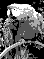
2 bit image
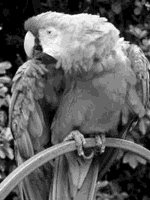
4 bit image
The image becomes more detailed, the greater the bit depth. Below, you can find an animation where a continuous gradient is drawn with an increasing number of combinations. They don’t always represent a real bit depth, but they highlight one thing really well: after a certain number of bit depth, the gain from more combinations is diminishing. The human eye can only distinguish so many shades, after a certain number, new shades won’t really matter.
Real examples and pitfalls
So far we at somewhat artificial samples of grayscale images. How does bit depth affect us in real life. Let’s look at fluorescent microscopy and western blots. In both cases, we measure a signal at a position. We transform this signal into image data. Let’s imagine we have a western blot with four bands. Each has a distinct intensity, and we want to transform these intensities into digital data. How does bit depth affect our signal?
| real intensity | 1 bit | 2 bit | |
|---|---|---|---|
| Band A | 100% | 1 | 11 |
| Band B | 75% | 1 | 10 |
| Band C | 50% | 0 | 01 |
| Band D | 25% | 0 | 00 |
As you can see, a bit depth of 1 bit is not sufficient to encode the information of our source in detail. If we were to analyze the 2 bit image, we would conclude, that protein A and B have the same intensity. C and D — we would conclude – might be lost, while they are still present in reality. So we can also think of bit depth as granularity. The more bits available — the finer our discrimination between signals. And while a high bit depth might not matter to the human eye, the information conveyed by more bits might play an important role in your analysis.
A similar case can be made in fluorescent microscopy. If you transform your source signal into an image of high bit depth, you can resolve a higher range of intensities later on. If your bit depth is too low, you might not be able to detect real differences between signals.
Also, your camera or microscope has to fit your data into a certain range. If your exposure is too high, the captured data will be treated as the “highest” combination. If we were to capture the western blot above for too long, all the bands would receive the value 1 (in 1 bit) and 11 (in 2 bit). Since our signal was higher than the possible range, it was clipped to the highest possible value (overexposed). If we were capturing the blot too short, we would end up with zeros: not enough signal would hit the sensor of our camera, and it would not detect a signal.
Histograms
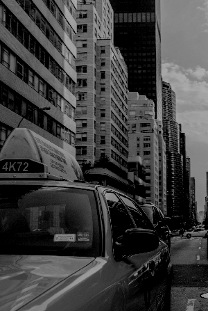
We can look at the distribution of intensities via histogram. In ImageJ, you can find this tool via Analyze → Histogram or Ctrl + H. As in statistics, you will get a diagram with the intensity on the x-, and the frequency on the y-axis. In ImageJ you can also hover over the data to see the exact numbers. Below, you can find the image of a taxi in New York. I’ve increased and decreased the brightness artificially, and added the histograms below. Also pay attention to the mode (the most frequent value).
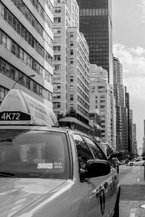
Original
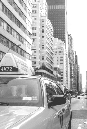
Brighter
Darker

Original (Histogram)
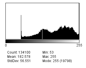
Brigther (Histogram)
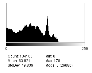
Darker (Histogram)
In the original histogram, you can see that the intensities are well spread out. There are some pixels with an intensity of zero (maybe the mirror of the taxi). You can also see a bright peak, probably due to the sky and buildings.
In the brighter (simulate overexposed) image, the modal is at intensity 255 (the maximum value for an 8 bit image). All the values above that are clipped to 255 since an 8 bit image cannot represent higher numbers. Details in areas that originally were bright are lost (e.g. the clouds in the sky).
In the darker (simulated underexposed) image, there is an abundant number of pixels with intensity 0. The bright intensities are missing and information in the dark areas is lost (e.g. the windows on the dark gray building).
When you work with images, you can check the histogram to evaluate the exposure. If the highest or lowest intensities have a large frequency, it might indicate inappropriate exposure. This can cause your analysis to lose precision or mask differences across brighter (or darker) areas. But if you are interested in a certain range (with a fine resolution), you might trade the loss of higher and lower intensities for that. In this case, accumulations of very high and very low pixels can be intended.
Bit depths in RGB
Now, after working with gray for a while, I want to make some remarks about color. When transforming color into digital data, we use a model to split color information into different intensities. In other words: we save a color as a mixture of red, green and blue. Each of these channels has a designated number of bits. For instance a 24bit RGB image has three channels made up of 8bit depth each. The principles above (e.g. clipping and resolution) apply to each channel individually. As such, each intensity has to be assigned to a “combination” of bits. I want to introduce one last artifact caused by too low bit depth: banding. Notice the harsh steps in the 8 bit parrots. The steps between intensities are still so large, that the human eye can see them easily. Therefore, we can see colored bands.
Original

8 bit RGB image with color banding
Outlook
We had a small look in the inner workings of digital images. We saw, how a continuous intensity has to be transformed into a “stepwise” format, in order for the computer to process it. So, what bit depth is the best? Let’s sum up what a higher bit depth allows us to do: we can either a) represent finer steps between intensities (e.g. we could go from 0 to 1 in 256 steps) or b) save a higher range of data (e.g. the range between 0 and 256 in steps of 1). With 16 bit we would have 65.536 steps available. But can you think of an example, where a 1 bit image would be suited best? If you’ve worked through the color model example, you might recall that we created a threshold — a categorization that assigns every pixel one of two categories. If we were to save this threshold as an image, a 1 bit file would be fine (since it has exactly two values).
In most cases however, the bit depth is given by the software you’re working with. Unfortunately you can’t “recover” signal that fell victim to a too low bit depth. As such, it is important to know the limitations of a too low bit depth and which artifacts can indicate, that the format is not appropriate. With that in mind, some knowledge about bit depth is a nice to have. It can sometimes be the case, that a piece of software only works with certain image formats (including a certain bit depth), and now you can judge about the potential issues of conversion.
Image sources
The original images can be found via the links below:
- Parrot by Ricardo Cancho Niemietz via Wikimedia Commons
- Taxis in new York by Lensicle via Flickr, licensed as CC-BY 2